4.2 Minimising errors (simple with help)
In this difficulty level, you train the same network as before, but a visual aid is provided. This aid slows down the performance as a lot of calculations are required here. However, it does show the best possible path to take to minimise errors and provides a deeper understanding of the optimisation algorithm.
Understanding the error of a neural network
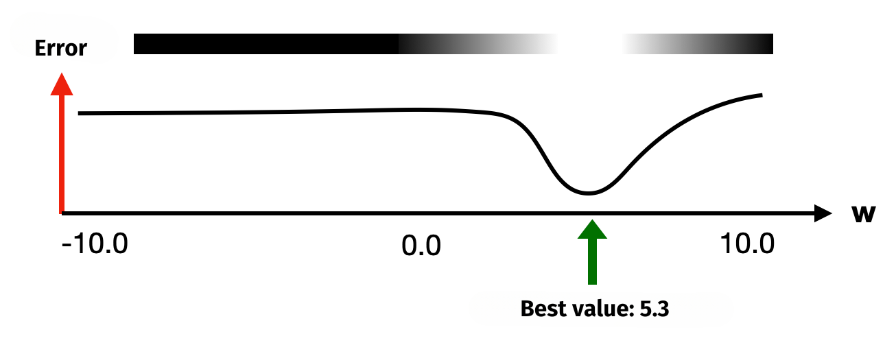
If a neural network only had a single adjustable weight w and no other knobs to turn, then different values for weight w would lead to different error values. However, there would certainly be a value for which the error would be the smallest. A theoretical example is given in the following illustration. This is what the network’s error might look like depending on weight value w:
Now, if there was a second adjustable weight, the error curve would be more difficult to depict. Instead of a curve, it would become a 3D surface. Weight w1 extends the axis to the left in the illustration, while weight w2 spans the axis diagonally to the rear-right. Finding the minimum error would mean descending into the lowest valley.
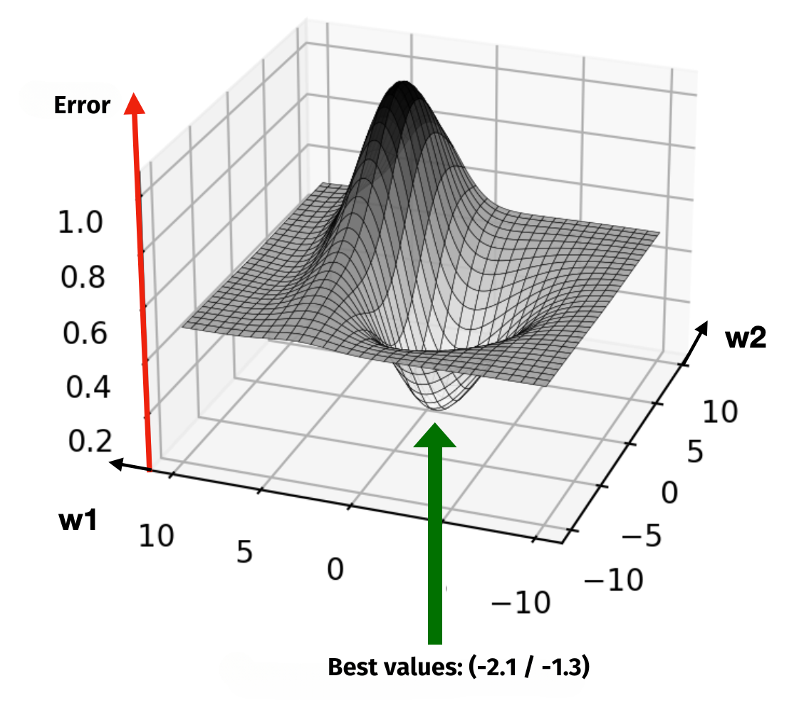
This “descent into the valley” is where the visualisation aid comes into play. The aim is always to reach the white area of the valleys, as the error is smaller there. The 3D landscape is shown from above as a 2D graphic in the upper right-hand corner. Since the neural network in the figure not only has two weights, but also a threshold value, it makes sense to start by adjusting the threshold first. This allows you to traverse the third dimension and then navigate into the white area afterward.
Instructions
- Use the checkboxes to select which training data should be loaded.
- Click
Newto select the preset values for a simple separation, a new randomly selected Boolean function or new random numbers as a data set. - Now click on the plus or minus signs in the figure to change the weights or the threshold value. The current error of the network is automatically displayed. If the error is small enough, you will receive a pop-up message with your required time. Use the plus or minus signs to move the small black circle within the graphical aid into as white an area as possible. The area might not be sufficient for the example data with random numbers.
- Click
Resetto undo all your current changes to the weights and threshold. - Click
Trainto start or resume training. - In the figure on the left, blue stands for negative values and red stands for positive values.
Task
Try out many different examples and minimise the network’s error for each one.
From the algorithmic perspective
In all the neural networks used on these pages, the backpropagation and gradient descent methods are used during training. These follow their own, rather complex strategy of reducing errors from back to front (i.e. backwards, hence “backpropagation”). The weights are adjusted layer by layer (from output to input) based on their influence on the error of the network. In purely algorithmic terms, the goal is also to “descend into valleys” as far as possible (there are actually purely mathematical solution methods for this). However, the valley analogy would only really be illustrative if the entire neural network only had two weights. For each additional weight and each additional threshold value, one more dimension is added. When neural networks with tens of thousands of neurons are trained, finding the deepest possible valley in a space with tens of thousands of dimensions becomes practically unimaginable. Nevertheless, it can be solved algorithmically, and thanks to modern PC hardware, very quickly at that.
To better understand the challenge of tuning 13 different parameters (i.e. weights and thresholds), you should definitely try the more difficult example on the next page!
Share this page