5.3 Images

Convolutional Neural Networks or: How can neural networks classify images?

A digital image consists of so-called pixels, which are nothing more than numerical values for a computer. These can, in turn, be processed as input data with a neural network. For the sake of simplicity, only greyscale images with a size of 5x5 pixels will be considered below, which means that each image consists of exactly 25 numbers ranging between 0 and 1.

To get a feel for what this page is about, it can be beneficial to use a proper application of image processing with artificial neural networks beforehand. Google Quickdraw is a good tool for this. It offers a small interactive program that tries to guess what you have drawn on the screen with the mouse. You’ll be given six tasks one after the other, such as: “Draw a street lamp in 19 seconds.” Within the available time, the program tries to recognise your drawing as accurately and quickly as possible. It does not matter whether you draw the image on the left, right, top, bottom, large, small, or tilted. It is usually recognised anyway.

A new network architecture

The following neural network in the interactive figure works in a similar way to the neural network used in Quickdraw – in a very simplified manner. It is a so-called convolutional neural network. In addition to the familiar components, it has three new concepts: a filter, a special layer called convolution, and another special layer called max pooling. To make it clear from the start: In neural networks on the scale of Google’s Quickdraw, these three new concepts are present not once, but multiple times throughout the network. A typical convolutional neural network consists of several to many layers of convolution and max pooling followed by a “regular” neural network of the type that we have learnt about so far. Even if this sounds complicated at first, the new layers only involve simple mathematical calculations that can be easily tracked in the interactive figure.

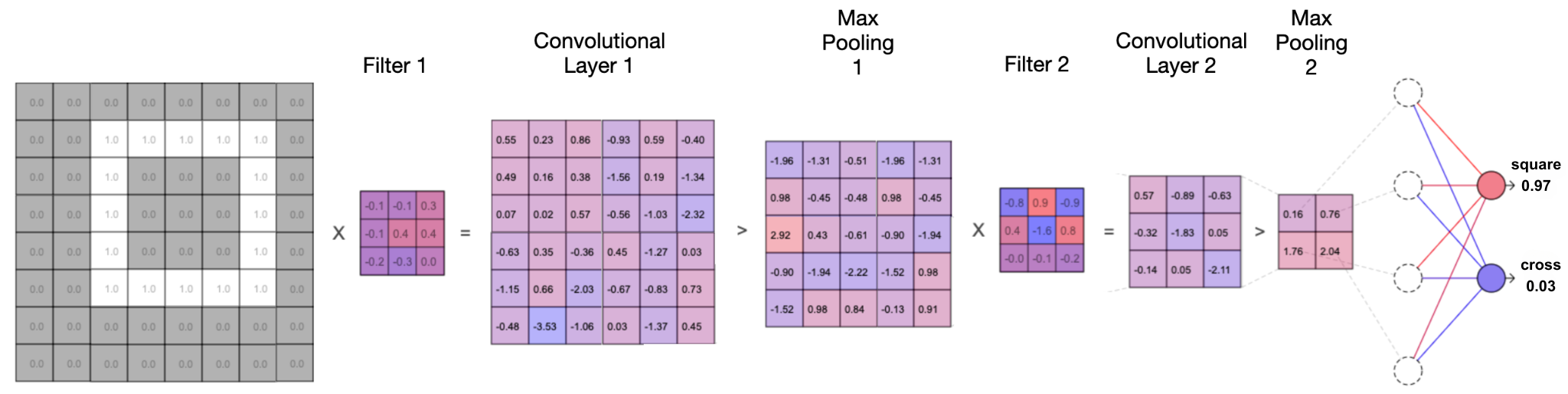
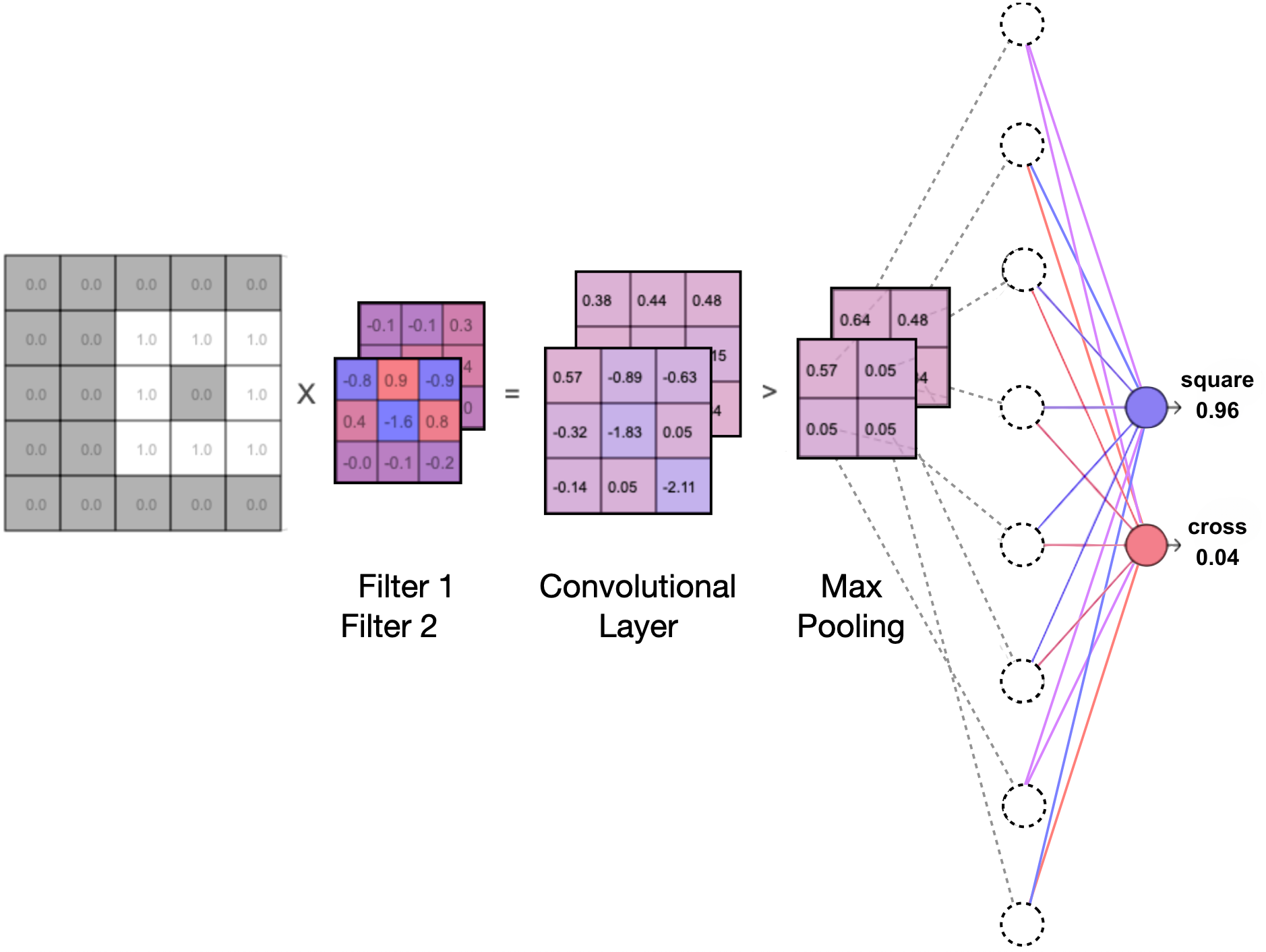
This page uses the simplest possible convolutional neural network so that it can be understood step by step. It consists of a single combination of convolution and max pooling and has just one filter. In addition, it can only classify images from two classes (in the example below: black and white) that are at most 5x5 pixels in size – truly a minimal example.

How it works

The filter consists of 3x3 numbers, which are trained and adjusted in addition to the eight regular weights and two thresholds. The filter slides from the top left to the bottom right across the input image, and at each step, it multiplies and adds up all the values with the corresponding pixel values. This process creates a smaller representation of the original image. A 2x2 window is then slid over this new image, and the maximum value within each window is extracted. In the end, the 5x5 grid becomes a 2x2 grid containing four values that now serve as input to the “regular” neural network.

Three different example data sets can be loaded in the interactive figure. The network can be trained with the displayed training data and tested with the test data at the bottom of the figure by clicking on a test image. Along with the calculations, you can also see the prediction of what the network thinks the input image is. In addition, the calculation of the network can be animated step by step.

More filters and larger networks

You might have noticed this in the first two examples: As the filter is also trained during training, it develops a pattern that is particularly effective at distinguishing features of the two classes. Often, a graphically visible structure such as a horizontal, vertical or diagonal line can be found in the filter – depending on the available training data.

Accordingly, the more filters there are in a neural network, the more features and structures can be identified. Essentially, a filter detects the presence of specific features in the form of numbers and passes it on to the next convolutional layer. This is why it makes a lot of sense to have as many filters as possible in order to be able to distinguish different classes based on various features and structures. While there are exactly 19 parameters in the minimal example given here (9 filter values, 8 weights, 2 thresholds), modern high-performance networks use more than 2 billion parameters for image classification. These networks often handle data sets with 1000 or more classes.

In principle, the above example can be extended stepwise by chaining more filters in series and simultaneously connecting more filters in parallel. Since all filters are created with random starting values, they are very likely to recognise different features in the images – especially when the data set is large enough, which is crucial for training neural networks anyway.

Relearning

A well-functioning convolutional neural network has many filters that skilfully pass the features of images to the right. After successful training, the filters work so well that it does not matter whether a vertical line is drawn on the right or left, in the centre, at the top, at the bottom, large or small. The information of the vertical line is still passed through the network to the right.

This makes it possible to freeze the front part (consisting of filters, convolution and max-pooling layers) if it works excellently, and only have the back part (the regular neural network) relearn. In other words, if you have a network that recognises apples and pears well, the front part of the network will have developed good filters to achieve this. You can now leave these filters unchanged and train the back part to output, for example, 1 0 for pears and 0 1 for plums, or 1 0 for images of ladybirds and 0 1 for images of caterpillars. This procedure (retraining an existing well-functioning network) is used, for example, in image projects of Google’s Teachable Machine.

Creative finale

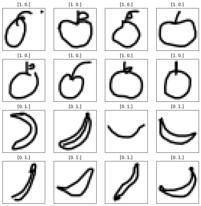
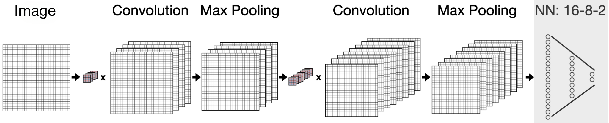
In the following, we’ll use a slightly larger convolutional neural network than in the example above to categorise drawings that you can make yourself into the classes of apple and banana. The pre-trained neural network was trained with images that are 28x28 pixels in size. The images come from the training data provided by Google Quick, Draw! and contain hand-drawn sketches of apples and bananas.

The neural network used here has 4 parallel filters in the first convolutional layer, followed by a max-pooling layer with a 2x2 window, then 8 parallel filters in the second convolutional layer, again followed by a max-pooling layer. The actual neural network comes last and consists of 16 neurons in the first layer, 8 neurons in the second layer and 2 output neurons.